Quantum Computing¶

Quantum Bit, Quantum Superposition, and Quantum Entanglement¶

Bit is a fundamental concept in classical computing and information. Quantum computing and quantum information are also based on similar conceptual quantum bit or qubit. Similar to the classical bits, which can be in the 0 state or the 1 state, the qubits have similar states.

Two possible quantum states are $|0\rangle$ and $|1\rangle$, or, this is similar to the classical bits 0 and 1. Here $|\rangle$ is the Dirac symbol that physicists prefer to use and in the following part, we will use Dirac symbol by default. Unlike classical bits, the qubit can be in a state other than concrete $|0\rangle$ and $|1\rangle$. Namely, it can also be in a linear superposition state of $|0\rangle$ and $|1\rangle$. In physics, we call it a quantum superposition state:

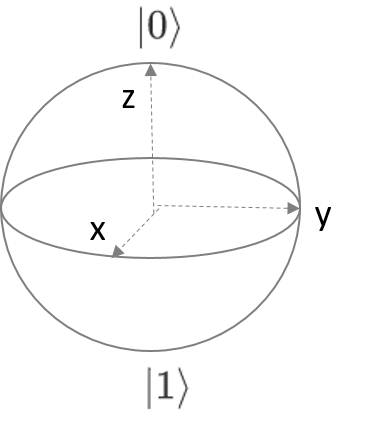
\[|\psi\rangle=\alpha |0\rangle +\beta |1\rangle.\]

Here $\alpha$ and $\beta$ are both complex numbers, and $|\alpha|^{2}+|\beta|^2=1$. Here $|0\rangle$ and $|1\rangle$ is the basis vector of our calculations. Mathematically, a two-dimensional complex vector of quantum bits can be formed in the basis vectors $|0\rangle$ and $|1\rangle$. In order to distinguish the qubit and the classical bit more intuitively, the classical bits 0 and 1 can be understood as the north and south poles of the earth, as shown in the figure, while the qubits $|\psi \rangle$ can be in the superposition state, which has an infinite number of possibilities. This state can be shown in Bloch’s ball as follows:

Considering implementing a complicated quantum computer, it is inevitable to involve a complex many-body quantum system. We use the direct product symbol $\otimes$ to describe the combination of two quantum systems as a separable composed quantum system, which can be generalized to quantum systems with more qubits. Let’s take a closer look at this case with two qubits as an example. For two qubits with individual quantum states of $|\psi_{1}\rangle$ and $|\psi_{2}\rangle$, they can form a composed system. From the perspective of composing a system, it can be described as $|\Psi\rangle=|\psi_{1}\rangle|\psi_{2}\rangle$, alternatively it can be expanded into:

\[\begin{split}|\Psi\rangle=|\psi_{1}\rangle\otimes|\psi_{2}\rangle \\ =\alpha_{1}\alpha_{2}|0_{1}\rangle|0_{2}\rangle +\alpha_{1}\beta_{2}|0_{1}\rangle|1_{2}\rangle+\beta_{1}\alpha_{2}|1_{1}\rangle|0_{2}\rangle+\beta_{1}\beta_{2}|1_{1}\rangle|1_{2}\rangle \\ =\alpha_{1}\alpha_{2}|00\rangle +\alpha_{1}\beta_{2}|01\rangle +\beta_{1}\alpha_{2}|10\rangle +\beta_{1}\beta_{2}|11\rangle\end{split}\]

Here we use the subscript to indicate the corresponding qubit, and ignore the direct product symbol $\otimes$ in the last row of the reduction. Our default qubit coordinates are 0,1,… from left to right respectively. The composite state $|\Psi\rangle$ of the two directly formed states is called the direct product state (separable state). In addition to these states in quantum systems, there is another kind of states that cannot be generated by direct products, such as a Bell state:

\[|\Psi_{Bell}\rangle=\frac{1}{\sqrt{2}}|00\rangle +\frac{1}{\sqrt{2}}|11\rangle\]

Such a state, in any case, cannot be decomposed into a direct product of two quantum states. We call such a state a quantum entangled state. As an important quantum resource, quantum entanglement is widely used in quantum computing and quantum communication.

The rules of the direct product can be understood from the following case. For two 2*2 matrices A and B defined as

\[\begin{split}\begin{matrix} A=\begin{bmatrix} A_{11} & A_{12}\\ A_{21} & A_{22} \end{bmatrix}, B=\begin{bmatrix} B_{11} & B_{12} \\ B_{21} & B_{22} \end{bmatrix} \end{matrix}\end{split}\]

In order to understand the direct product, we can perform the product from a matrix perspective. Define quantum states $|0rangle=(1,0)^{T}$ and $|1rangle=(0,1)^{T}$. Here T is the transpose operator. Then

\[\begin{split} \begin{align} A\otimes B &=\begin{matrix} \begin{bmatrix} A_{11}B & A_{12}B\\ A_{21}B & A_{22}B \end{bmatrix} \end{matrix} \\ &=\begin{matrix} \begin{bmatrix} A_{11}*B_{11} &A_{11}*B_{12} &A_{12}*B_{11} & A_{12}*B_{12} \\ A_{11}*B_{21} &A_{11}*B_{22} &A_{12}*B_{21} & A_{12}*B_{22} \\ A_{21}*B_{11} &A_{21}*B_{12} &A_{22}*B_{11} & A_{22}*B_{12} \\ A_{21}*B_{21} &A_{21}*B_{22} &A_{22}*B_{21} & A_{22}*B_{22} \\ \end{bmatrix} \end{matrix} \end{align}\end{split}\]

Based on this rule, we can get it easily.

\[\begin{split}\begin{matrix} |00\rangle=\begin{bmatrix} 1 \\ 0 \\ 0 \\ 0 \end{bmatrix}, |01\rangle=\begin{bmatrix} 0 \\ 1 \\ 0 \\ 0 \end{bmatrix}, |10\rangle=\begin{bmatrix} 0 \\ 0 \\ 1 \\ 0 \end{bmatrix}, |11\rangle=\begin{bmatrix} 0 \\ 0 \\ 0 \\ 1 \end{bmatrix} \end{matrix}\end{split}\]

Then we can write,

\[\begin{split}\begin{matrix} |\Psi\rangle=\begin{bmatrix} \alpha_1\alpha_2 \\ \alpha_1\beta_1 \\ \beta_1\alpha_2 \\ \beta_1\beta_2 \end{bmatrix}, |\Psi_{Bell}\rangle=\begin{bmatrix} \frac{1}{\sqrt{2}} \\ 0 \\ 0 \\ \frac{1}{\sqrt{2}} \end{bmatrix} \end{matrix}\end{split}\]

Quantum State Evolution and Quantum Gate Operation¶

In a closed system, the evolution of a quantum state can be described by a unitary transformation. The quantum state at t1 instance $|\psi({t1})\rangle$ can be transformed to $|\psi({t1})\rangle$ by a unitary operator U(unitary operator), which is only dependent on time t1 and t2

\[|\psi(t2)\rangle=U(t1,t2) |\psi(t1)\rangle\]

To be concrete, the evolution of a closed system quantum state obeys the Schrödinger equation, that is,

\[i\hbar\frac{d |\psi\rangle}{d t}=H |\psi\rangle.\]

In this equation, $\hbar$ is the Planck constant in physics, and H is the Hamiltonian of the system. Simply speaking, a quantum system, if you know its initial state $|\psi_{t=0}\rangle$, and Hamiltonian, you can get $|\psi_{t}\rangle$ at arbitrary t by solving the Schrödinger equation. In general, similar to classical machine initialization, a single qubit state is initialized at $|0\rangle$, that is the state of the system after initialization is generally deterministic, so the most important thing is to construct the system’s Hamiltonian. From a computational point of view, the Hamiltonian evolution can be decomposed into a combination of various single-bit and two-bits quantum. Analogy to classical computers, starting from some gate collections (such as OR gates, AND gates and NAND gate), you can combine and complete any classical calculation process. Similarly, a series of complex quantum calculations can also be achieved by constructing a corresponding complex Hamiltonian, and then can be achieved by decomposing into a series of quantum gates. Theoretical calculations show that a single-bit gate and a two-bit gate CNOT set can constitute a complex gate of arbitrary quantum computation.

Commonly used single quantum bit gates are mainly Pauli operators X, Y, and Z, and Hadamard gate H, and $\frac{\pi}{4}$ and $\frac{\pi}{8}$ phase gates, S and T gates. Their corresponding matrices are:

\[\begin{split}\begin{matrix} X=\begin{bmatrix} 0 & 1\\ 1 & 0 \\ \end{bmatrix}, Y=\begin{bmatrix} 0 & -i \\ i & 0 \end{bmatrix}, Z=\begin{bmatrix} 1 & 0 \\ 0 & -1 \\ \end{bmatrix},\\ H=\frac{1}{\sqrt{2}}\begin{bmatrix} 1 &1 \\ 1 &-1 \end{bmatrix},S=\begin{bmatrix} 1 & 0 \\ 0 & i \\ \end{bmatrix},T=\begin{bmatrix} 1 & 0 \\ 0 & e^{i\pi/4} \\ \end{bmatrix} \end{matrix}\end{split}\]

For single-qubit gates, we take the X gate and the H gate as examples. An X gate can flip the input state.

\[|\psi\rangle=\alpha |0\rangle +\beta |1\rangle.\]

\[\begin{split}\begin{align} X|\psi\rangle &=\begin{matrix} \begin{bmatrix} 0 & 1 \\ 1 & 0 \end{bmatrix}*\begin{bmatrix} \alpha \\ \beta \end{bmatrix} =\begin{bmatrix} \beta \\ \alpha \end{bmatrix} =\alpha|1\rangle+\beta|0\rangle \\ \end{matrix} \end{align}\end{split}\]

A Hadamard gate can be used to prepare superposition states and transform basis vectors.

\[\begin{split}\begin{align} H|0 \rangle &=\begin{matrix} \frac{1}{\sqrt{2}} \begin{bmatrix} 1 & 1 \\ 1 & -1 \end{bmatrix} *\begin{bmatrix} 1 \\ 0 \end{bmatrix} =\frac{1}{\sqrt{2}} \begin{bmatrix} 1 \\ 1 \end{bmatrix} =\frac{1}{\sqrt{2}}(|0\rangle+|1\rangle )\\ \end{matrix} \end{align}\end{split}\]

\[\begin{split}\begin{align} H|1 \rangle &=\begin{matrix} \frac{1}{\sqrt{2}} \begin{bmatrix} 1 & 1 \\ 1 & -1 \end{bmatrix} *\begin{bmatrix} 1 \\ 0 \end{bmatrix} =\frac{1}{\sqrt{2}} \begin{bmatrix} 1 \\ 1 \end{bmatrix} =\frac{1}{\sqrt{2}}(|0\rangle-|1\rangle )\\ \end{matrix} \end{align}\end{split}\]

For two qubit gates, we focus on the CNOT gate, that is, a control-flip gate. It is generally assumed that the first qubit is the control bit and the second qubit is the target qubit. Then, if and only if the first bit is the quantum state $|1\rangle$, the second bit performs the flip operation, that is, the X operation. The CNOT gate in matrix form is:

\[\begin{split}\begin{matrix} CNOT=CX=\begin{bmatrix} 1 & 0 & 0 & 0 \\ 0 & 1 & 0 & 0 \\ 0 & 0 & 0 & 1 \\ 0 & 0 & 1 & 0 \end{bmatrix} \end{matrix}\end{split}\]

It is easy to verify the following function:

\[\begin{split}\begin{matrix} CNOT |00\rangle=\begin{bmatrix} 1 & 0 & 0 & 0 \\ 0 & 1 & 0 & 0 \\ 0 & 0 & 0 & 1 \\ 0 & 0 & 1 & 0 \end{bmatrix}*\begin{bmatrix} 1 \\ 0 \\ 0 \\ 0 \end{bmatrix}=\begin{bmatrix} 1 \\ 0 \\ 0 \\ 0 \end{bmatrix}=|00\rangle, \\ CNOT |01\rangle=\begin{bmatrix} 1 & 0 & 0 & 0 \\ 0 & 1 & 0 & 0 \\ 0 & 0 & 0 & 1 \\ 0 & 0 & 1 & 0 \end{bmatrix}*\begin{bmatrix} 0 \\ 1 \\ 0 \\ 0 \end{bmatrix}=\begin{bmatrix} 0 \\ 1 \\ 0 \\ 0 \end{bmatrix}=|01\rangle, \\ CNOT |10\rangle=\begin{bmatrix} 1 & 0 & 0 & 0 \\ 0 & 1 & 0 & 0 \\ 0 & 0 & 0 & 1 \\ 0 & 0 & 1 & 0 \end{bmatrix}*\begin{bmatrix} 0 \\ 0 \\ 1 \\ 0 \end{bmatrix}=\begin{bmatrix} 0 \\ 0 \\ 0 \\ 1 \end{bmatrix}=|11\rangle, \\ CNOT |11\rangle=\begin{bmatrix} 1 & 0 & 0 & 0 \\ 0 & 1 & 0 & 0 \\ 0 & 0 & 0 & 1 \\ 0 & 0 & 1 & 0 \end{bmatrix}*\begin{bmatrix} 0 \\ 0 \\ 0 \\ 1 \end{bmatrix}=\begin{bmatrix} 0 \\ 0 \\ 1 \\ 0 \end{bmatrix}=|10\rangle \end{matrix}\end{split}\]

The CNOT gate is indispensable in the operation of two qubits to prepare the quantum entangled state!

Quantum Circuit¶

In order to demonstrate a complex quantum computing process, we choose to show two typical quantum circuits: the preparation of Bell state and quantum state teleportation.

The preparation of Bell entangled state

The preparation of the Bell state requires two qubits, assuming the initial state of qubits is $\psi_{0}=|00\rangle$,

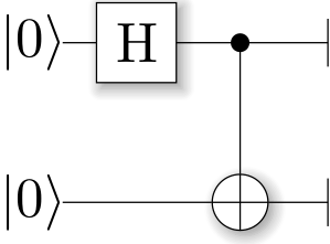
First, apply a Hadamard gate operation to Qubit1, the composed system becomes

\[\begin{split}\begin{align} \psi_{1}&=\frac{1}{\sqrt{2}}(|0\rangle+|1\rangle)|0\rangle \\ &=\frac{1}{\sqrt{2}}(|00\rangle+|10\rangle) \end{align}\end{split}\]

Second, taking qubit1 as the control bit and qubit2 as the target bit, applying the CNOT gate, the system evolves to

\[\begin{align} \psi_{2} &=\frac{1}{\sqrt{2}}(|00\rangle+|11\rangle) \end{align}\]

Third, a Bell entangled state was prepared by the Hadamard gate and the CNOT gate. By changing the initial state combination, we can prepare other additional 3 Bell states. It is easy to verify that the following four corresponding Bell states can be constructed by different combinations.

\[\begin{split}\begin{align} |00\rangle \rightarrow \Phi^{+} &=\frac{1}{\sqrt{2}}(|00\rangle+|11\rangle), \\ |10\rangle \rightarrow \Phi^{-} &=\frac{1}{\sqrt{2}}(|00\rangle-|11\rangle), \\ |01\rangle \rightarrow \phi^{+} &=\frac{1}{\sqrt{2}}(|01\rangle+|10\rangle), \\ |11\rangle \rightarrow \phi^{-} &=\frac{1}{\sqrt{2}}(|01\rangle-|10\rangle), \\ \end{align}\end{split}\]

Fourth, here, different symbols are used to distinguish different Bell states. Entanglement represents a non-local relationship. In terms of $\Phi^{+}$, ideally, if the state of qubit1 is measured to be state 0, the quantum state of qubit2 will also collapse to state 0. If the qubit1 measurement is 1, then qubit2 will also collapse to quantum state 1.

In experiments, correlation measurements and quantum state tomography are required to show entangled states. However, as the system increases, the matrix element index of the quantum state increases exponentially, and the quantum state tomography is difficult to operate theoretically and experimentally. Therefore, the entanglement measure of multi-body complex system is still a topic worth studying.

Quantum state teleportation

Entanglement can be used as a resource for quantum teleportation. Here, we use the quantum circuit to demonstrate quantum teleportation.

First, suppose there is a quantum state in Alice’s position that we want to transport to Bob. Without loss of generality, we describe this state with a Dirac symbol as

\[|\psi\rangle_{C}=\alpha|0_{C}\rangle +\beta |1_{C}\rangle\]

Second, the protocol assumes that Alice and Bob are initially in a maximally entangled Bell state. This entangled state can be one of the following four types. We choose one in advance

\[\begin{split}|\Phi^{+}\rangle_{AB} =\frac{1}{\sqrt{2}}(|0_{A}0_{B}\rangle+|1_{A}1_{B}\rangle),\\ |\Phi^{-}\rangle_{AB} =\frac{1}{\sqrt{2}}(|0_{A}0_{B}\rangle+|1_{A}1_{B}\rangle),\\ |\phi^{+}\rangle_{AB} =\frac{1}{\sqrt{2}}(|0_{A}1_{B}\rangle+|1_{A}0_{B}\rangle),\\ |\phi^{-}\rangle_{AB} =\frac{1}{\sqrt{2}}(|0_{A}1_{B}\rangle-|1_{A}0_{B}\rangle),\\\end{split}\]

We assume that Alice and Bob share a maximally entangled state $|\Phi^{+}\rangle_{AB}$ at the very beginning.

Now, Alice has two quantum states, one is the state C to be transported, the other is the state A entangled with Bob, and Bob currently is only in the quantum state B (which is also part of the entangled state). Consider the entire system together, we obtain the three qubits which can be described as,

\[\begin{split}\begin{align} |\psi_{0}\rangle=|\psi\rangle_{AB}|\psi\rangle_{C} &=\frac{1}{\sqrt{2}}(|0_{A}0_{B}\rangle+|1_{A}1_{B}\rangle) (\alpha|0_{C}\rangle+\beta|1_{C}\rangle) \\ &=\frac{1}{\sqrt{2}}\{\alpha(|0_{A}0_{B}0_{C}\rangle + |1_{A}1_{B}0_{C}\rangle) +\beta(|0_A0_B1_C\rangle +|1_A1_B1_C\rangle)\} \end{align}\end{split}\]

One step further, taking into account that the subsequent measurements are measured under the Bell measurement basis, the state of the system can be expanded in the Bell state, using the following relationship,

\[\begin{split}|00\rangle=\frac{1}{\sqrt{2}}(|\Psi^{+}\rangle+|\Psi^{-}\rangle),\\ |11\rangle=\frac{1}{\sqrt{2}}(|\Psi^{+}\rangle-|\Psi^{-}\rangle),\\ |01\rangle=\frac{1}{\sqrt{2}}(|\psi^{+}\rangle+|\psi^{-}\rangle),\\ |10\rangle=\frac{1}{\sqrt{2}}(|\psi^{+}\rangle-|\psi^{-}\rangle).\\\end{split}\]

Keep Bob’s partial quantum state B unchanged and focus on Alice’s part of the quantum state A and the quantum state C, the system can be written as,

\[\begin{split}\begin{align} |\psi_{0}\rangle &=\frac{1}{\sqrt{2}}\{\alpha(|0_{A}0_{B}0_{C}\rangle + |1_{A}1_{B}0_{C}\rangle) +\beta(|0_A0_B1_C\rangle +|1_A1_B1_C\rangle)\} \\ &=\frac{1}{\sqrt{2}}\{\frac{\alpha}{\sqrt{2}}(|\Psi^{+}_{AC}\rangle+|\Psi^{-}_{AC}\rangle)|0_{B}\rangle + \frac{\alpha}{\sqrt{2}}(|\psi^{+}_{AC}\rangle-|\psi^{-}_{AC}\rangle)|1_{B}\rangle +\\&\qquad\frac{\beta}{\sqrt{2}} (|\psi^{+}_{AC}\rangle+|\psi^{-}_{AC}\rangle)|0_{B}\rangle +\frac{\beta}{\sqrt{2}}(|\Psi^{+}_{AC}\rangle-|\Psi^{-}_{AC}\rangle)|1_{B}\rangle \} \\ &=\frac{1}{2}\{|\Psi^{+}_{AC}\rangle(\alpha|0_B\rangle+\beta|1_B\rangle) + |\Psi^{-}_{AC}\rangle(\alpha|0_B\rangle-\beta|1_B\rangle) + \\ &\qquad |\psi^{+}_{AC}\rangle(\beta|0_B\rangle)+\alpha|1_B\rangle) + |\psi^{+}_{AC}\rangle(\beta|0_B\rangle)-\alpha|1_B\rangle)\} \end{align}\end{split}\]

It can be clearly seen that if measured in the Bell basis, the quantum state B on Bob can be recovered by the corresponding operation according to the measurement results. So, we can do the corresponding quantum operations on Bob based on the results of Bell measurements.

The Bell state of Alice is measured as $|\Psi^{+}_{AC}\rangle$, then the quantum state of B at Bob collapses to $\alpha|0\rangle+\beta|1\rangle$, this state is to be transported to Bob, so Bob does nothing.
The Bell state of Alice is measured as $|\Psi^{-}_{AC}\rangle$, then the quantum state of B at Bob collapses to $\alpha|0\rangle-\beta|1\rangle$, which requires a Z operation and turns it into $\alpha|0\rangle+\beta|1\rangle$.
The Bell state of Alice is measured as $|\psi^{+}_{AC}\rangle$, then the quantum state of B at Bob collapses to $\beta|0\rangle+\alpha|1\rangle$, which requires an X operation and turns it into $\alpha|0\rangle+\beta|1\rangle$.
The Bell state of Alice is measured as $|\psi^{-}_{AC}$, then the quantum state of B at Bob collapses to $\beta|0\rangle-\alpha|1\rangle$. Here, an X gate operation is applied and transfer the state into $\alpha|0\rangle-\beta|1\rangle$, followed by a Z gate, which convert the quantum state to $\alpha|0\rangle+\beta|1\rangle$.

In the experiment, considering the complexity of measuring the entangled state and the reversibility of quantum computing, the inverse operation of preparing the entangled state is applied. That is, first apply the CNOT gate operation, then apply the Hadamard gate,

It should be noted that the qubit C is the control bit and A is the target bit. Through this unitary transformation, the entangled state can be converted into a measurement basis vector of the state 0 and 1, which can be measured in the experimental system. This is a one-to-one mapping, we specify the following relationship as,

\[\begin{split}\begin{align} \Phi^{+}_{AC} &=\frac{1}{\sqrt{2}}(|0_A0_C\rangle+|1_A1_C\rangle) \rightarrow |0_A0_C\rangle, \\ \Phi^{-}_{AC} &=\frac{1}{\sqrt{2}}(|0_A0_C\rangle-|1_A1_C\rangle) \rightarrow |0_A1_C\rangle, \\ \phi^{+}_{AC} &=\frac{1}{\sqrt{2}}(|0_A1_C\rangle+|1_A0_C\rangle) \rightarrow |1_A0_C\rangle, \\ \phi^{-}_{AC} &=\frac{1}{\sqrt{2}}(|0_A1_C\rangle-|1_A0_C\rangle) \rightarrow |1_A1_C\rangle, \\ \end{align}\end{split}\]

The quantum teleportation circuit diagram is as follows:

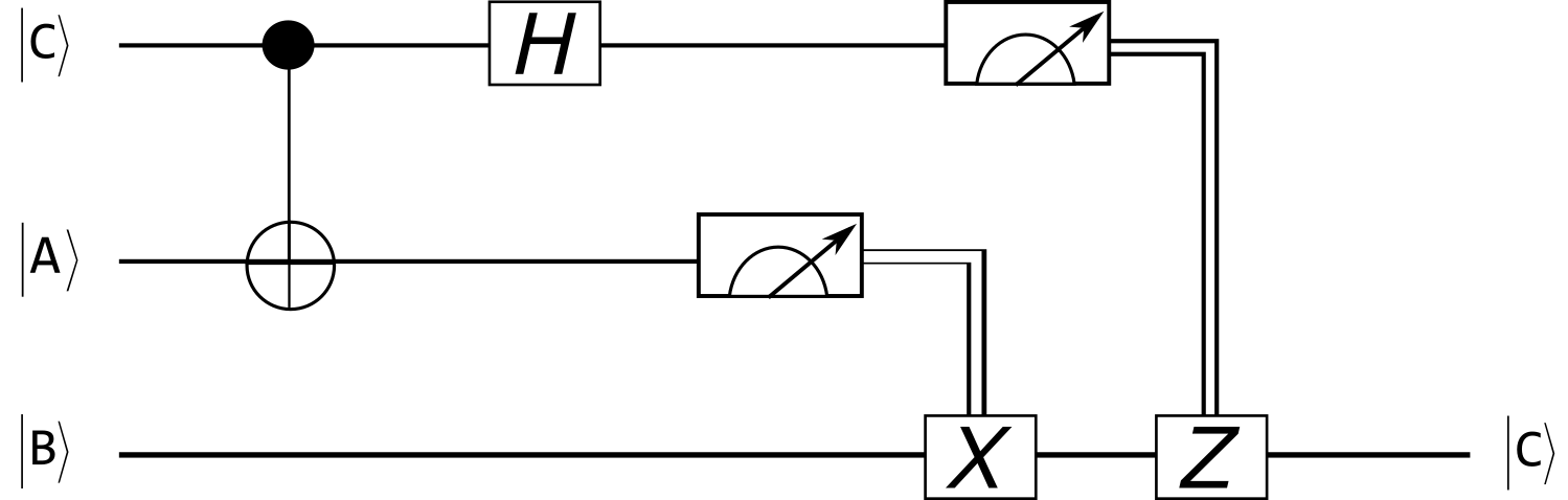
According to the above one-to-one mapping relationship, we can get,

When the measurement result is $|\psi\rangle=|0_{A}0_{C}\rangle$, no operation is required on the quantum state B, and the quantum state C is obtained naturally.
When the measurement result is $|\psi\rangle=|0_{A}1_{C}\rangle$, a Z gate needs to be manipulated on the quantum state B.
When the measurement result is $|\psi\rangle=|1_{A}0_{C}\rangle$, an X gate needs to be manipulated on the quantum state B.
When the measurement result is $|\psi\rangle=|1_{A}1_{C}\rangle$, an X gate needs to be operated first, followed by a Z gate on the quantum state B.

The Research Progress on Quantum Computer Hardware Implementation Platform¶

Quantum computing and quantum information are more than just a set of mathematical descriptions. Scientists are convinced that machines that process quantum information should be created in nature. However, the implementation of quantum circuits, quantum algorithms, and quantum communication systems in the experiment still has great challenges in engineering. We analyze more mainstream physical systems that realize quantum computing, ion trap quantum computing systems, and superconducting quantum computing systems from our perspective. Since there are a large number of groups of scientists who study these systems worldwide, we will focus on some of the basic elements of quantum computing. We hope that interested readers will read more in-depth and more generic introductions.

It is considered that what requirements are for a physical system to be implemented as a quantum computer. The most basic requirement is to have a qubit as a two-level system. In order to construct a quantum computer, in addition to being a qubit, the physical system should be able to maintain the systems’ quantum properties for a long time. Besides, we also hope that the quantum computer can work according to our expectations – in other words – controllable quantum manipulations or quantum evolutions. Of course, we also need high-fidelity state initialization and final state measurements. In summary, we need to satisfy the following necessary conditions to achieve universal quantum computing.

High fidelity qubit initialization
Long coherence time
Universal quantum gate operation
Effective quantum state measurement
Scalable quantum computing system

At present, the above five rules have been extended to seven, and we omitted the detailed information here. According to the above rules and the current research status, it has been widely believed that at least ion-trapped systems and superconducting circuit systems are promising platforms to achieve universal quantum computing.